2022-01 : Fluid Chemical Dynamics Simulation on GPU

I came up with this idea immediatly after learning about rate of reaction in a chemistry class I took.
Around the same time or right before, I came across several fluid simulation videos on youtube. Then, I thought to myself, since chemical reaction - i.e. rate of change of concentration of the substances - in liquid and gas phases are dictated by the rate laws which I just learnt how to calculate, can I just combine fluid dynamics and chemistry to simulate the chemical reaction of liquids as they also move around in the space? Thus, the fluid chemical dynamics simulation project is born.

I choose to use Jos Stam's algorithm published in 2003 as a starting point for the fluid dynamics component, since it is one of the simplest, have a youtuber who made a tutorial video for it, and deemed by me sufficiently realistic for simulating areas of different concentration in a solution.

I put together a simulation in JavaScript following the paper and the video, then added multiple concentration array to represent different substances soluted in the liquid. I then added a chemical reaction step running after the fluid simulation in each tick.

Click to see CPU simulation in action

Then I thought, can I make it even greater? Is it possible to simulate a bigger (finer detailed) space? I figured I must utilize the parallel computing powress of the GPU.
I refactored my code to run on kernels of GPU.js, a package that me write code in JavaScript to run on the GPU all on the web browser.

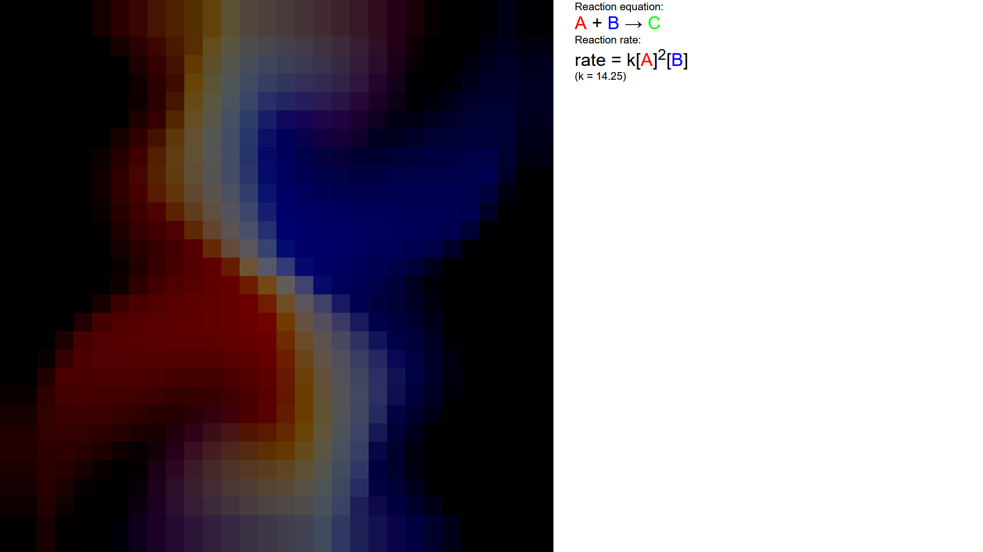
I changed up the reaction rule a little bit to reflect a different topic I learnt from the same chapter of rate of reaction chemistry class.

Click to see GPU simulation in action (Chrome, Edge)

Note: some browsers, mobile devices, or older computers does not support certain infrastructure code that GPU.js runs on. If you can't see the simulation, see this video below.

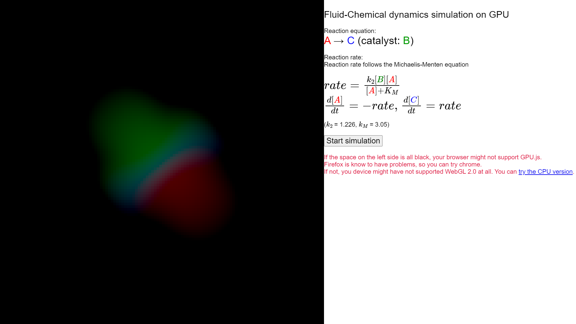
Around the same time, I showed this project to prof. Kyle Belozerov, my professor in the chemistry class I was in. He encouraged me to go deeper, and suggested me to try simulating the famous Belousov-Zhabotinsky Reaction.
The Belousov-Zhabotinsky Reaction (B-Z Reaction) is a phenomena created from a system of multiple individual reactions. It causes the system to express a periodic behaviour of repeatedly creating and then consuming the 3 key participants, displayed visually as beautiful blue and orange waves on a shallow plate.

Now the mechanism of the B-Z reaction is not fully known. The source I choose to cite describe the system as 5 fundamental reactions:

\[ \begin{aligned} (1) & \hspace{1em} & A + Y & \rightarrow & X + P & \hspace{3em} & rate = & 1.28[A][Y] \\ (2) & \hspace{1em} & X + Y & \rightarrow & 2P & \hspace{3em} & rate = & 2.4 \cdot 10^{6}[X][Y] \\ (3) & \hspace{1em} & A + X & \rightarrow & 2X + 2Z & \hspace{3em} & rate = & 33.6[A][X] \\ (4) & \hspace{1em} & 2X & \rightarrow & A + P & \hspace{3em} & rate = & 3 \cdot 10^{3} [X]^{2} \\ (5) & \hspace{1em} & B + Z & \rightarrow & Y & \hspace{3em} & rate = & 1.00[B][Z] \\ \end{aligned} \] Where letters standing for compounds: \[ \begin{aligned} A & \hspace{1em} & BrO_{3}^{-} \\ B & \hspace{1em} & Oxidizable \\ P & \hspace{1em} & HBrO \\ X & \hspace{1em} & HBrO_{2} \\ Y & \hspace{1em} & Br^{-} \\ Z & \hspace{1em} & Ce^{4+} \\ \end{aligned} \]

This can be viewed as a system of 1st order ordinary differential equations. Where the rate of change of the chemical's concentrations is dependant on the concentrations values. Where the first derivative with respect to time of each of the chemicals is dictated by the reaction rate functions. For example: \[ \begin{aligned} \frac{d[A]}{dt} & = (4) - (1) - (3) \\ & = 3 \cdot 10^{3} [X]^{2} - 33.6[A][X] - 1.28[A][Y] \\ \frac{d[Z]}{dt} & = 2 \cdot (3) - (5) \\ & = 2 \cdot 33.6[A][X] -1.00[B][Z] \end{aligned} \] Where the rate is added (positive) if the chemical is a product in that reaction, and subtracted (negative) if it is a reactant of the reaction.

These can all be combined to the vector function notation: \[ \frac{ds}{dt} = R(s) \] Where \(s\) is a vector of \([[A], [B], [P], [X], [Y], [Z]]\), and \(R(s)\) is the aggregate of all the reaction rate functions above.

Here, we cannot simply use an explicit method to propagete the system, since the large reaction rate constant of (2) and (4) giving a huge derivative (of concenctration with respect to time) value will cause the concentration value in a cell to become negative, which is physically impossible! This is known as a stiff differential equation.
Thus, just like solving for diffusion in the fluid dynamics part of the simulation, we will need to use an implicit method. An implicit method asks the question: "what is the value of the state of the system that, when rewinded h time units, will get us the current state?" They ensure the state cannot be negative.
Here I just choose the simplest one - the Implicit Euler method - which mathematically looks like this:

To solve the DE: \[ \frac{ds}{dt} = R(s) \] We do: \[ s_1 = s_0 + h \cdot R(s_1) \]

Where \(h\) is the difference in time between the two ticks.
It is an implicit method since \( s_1 \), the state of the system at the next time stop, exists on both sides of the equation and is a value we need to solve for instead of computing directly.

However, in here the state \(s\) is a vector 6 elements, one for the concentration of each specie of chemical compound.
We will essentially be solving a system of 6 non-linear equations.
Let's write the problem statement as this: \[ 0 = x - s_0 - h \cdot R(x) \] Here we want to solve for the unknown \(x\) which is the \( s_1 \) of above.

Thus, we can use the multivariate version of the Newton-Raphson method to find the roots of the function which is right hand side! \[ F(x) = x - s_0 - h \cdot R(x) \]

The multivariate Newton-Raphson method is as follows: \[ x_{n+1} = x_n - J(x_n)^{-1}F(x_n) \] Where \(J(x_n)\) is the jacobian matrix (derivate of a multivariate/vector function) of \(F(x)\). Start with an \(x_0\) and iterate until converge.
We can use \(s_0\) (concentration vector of the current tick) as the starting point \(x_0\)

To use the Newton-Raphson method, we need to derive the Jacobian matrix: \[ \begin{aligned} J(x) & = \frac{\partial F(x)}{\partial x} \\ & = \frac{\partial}{\partial x} (x - s_0 - hR(x)) \\ & = \frac{\partial}{\partial x} (x) - \frac{\partial}{\partial x}(s_0) - \frac{\partial}{\partial x}(hR(x)) \\ & = I_n - h \cdot \frac{\partial}{\partial x}R(x) \end{aligned} \] Since \(s_0\) is a constant, and the Jacobian of the identity vector function is just the identity matrix of the same dimension \(I_n\).

Finding the Jacobian of the aggregate rate function is quite trivial programatically as it is just a multivariate polynomial. Now all we need to do is to code up the function along with implementing a matrix inversion algorithm to run on the GPU.

And, success!

For rendering, I assigned the 3 color channels to represent the concentrations of \(HBrO_{2}\), \(Br^{-}\), and \(Ce^{4+}\). The higher the concentration of that chemical, the higher that color's value in the cell.
There are quite a few more kinks to iron out, but the simulation is working properly.
In the future I would want to explore more advance ways to doing this simulation, such as using the Lattice Boltzmann method for fluid dynamics, or using higher order Runge-Kutta methods to solve for the concentrations.